Math intuitions on variance
This is a supplement to High Variance Management, where I build some intuition on the different probability distributions involved. Please read that post before reading this one.
The normal and Gumbel probability distributions
We can develop some intuitions for these concepts using a simple probability model of Broadway and Hollywood. I'll use Julia to simulate distributions and plot them:
using Random, Distributions, Plots
plotly()
Random.seed!(123)
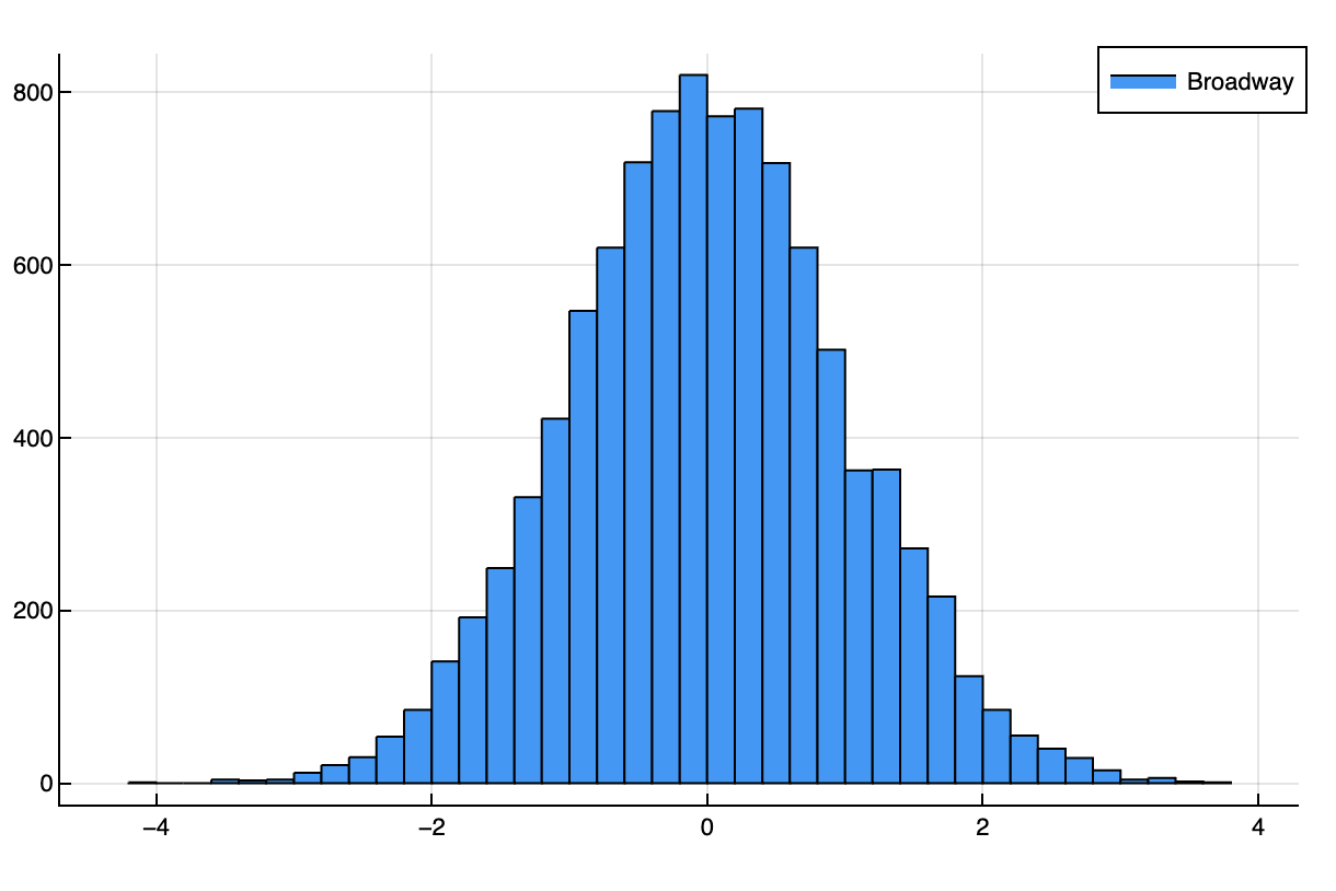
Let's assume that the quality of a given take from an actor follows a normal distribution with zero mean and variance of one, Normal(0, 1). This is a way of modeling the following intuitions:
- Most takes are close to the mean, which we pick to be zero.
- While there are some great takes (with quality higher than 1 or 2), they are rare.
- You get as many bad takes as good takes around the mean (the distribution is symmetric).
In Broadway, each take is the scene. So, how a scene goes looks like directly sampling from a normal distribution:
broadway = Normal(0, 1)
broadway_sample = rand(broadway, 10000)
histogram(broadway_sample, bins=50, label="Broadway")
In Hollywood, we can do two things differently:
- We encourage actors to take more risks. This makes it more likely that they produce good takes and bad ones. We are going to model this as moving the standard deviation to
1.5. - We do 10 takes (
n_takes = 10) and and pick the best one (maximum):hollywood = Normal(0, 1.5) n_samples = 10000 n_takes = 10 hollywood_sample = zeros(n_samples) for i in 1:n_samples hollywood_sample[i] = maximum(rand(hollywood, n_takes)) end histogram!(hollywood_sample, bins=50, label="Hollywood")
Here is how the new Hollywood distribution compares with the Broadway one:
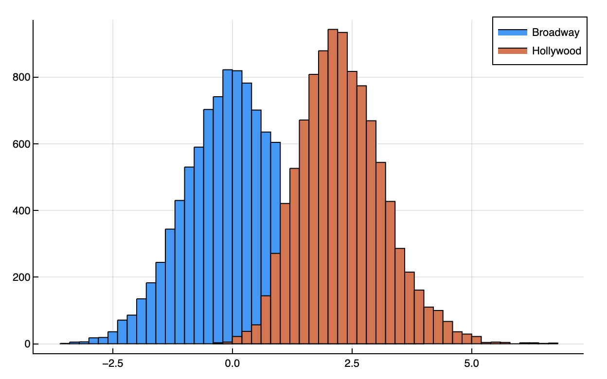
According to this toy model, Hollywood's resulting product can be much better:
- Your mean shot is much better. The Hollywood distribution is centered to the right of 0, with mean at 2.3, more than 2 standard deviations away from Broadway.
- You avoid almost all bad takes. Almost every Hollywood datapoint is to the right of zero, better than half of Broadway's datapoints. If you take the best of 10, the probability you get a negative number is
1/2^10 ≈ 0.1%. - You get some phenomenal shots. The Hollywood distribution goes all the way to 5, of which there are almost none in the Broadway distribution.
You can only do this when you lean into the variance. And you can only do that if there is no cost to bad takes.
The Hollywood distribution is similar to a Gumbel distribution which approximates taking the maximum of N samples of a normal distribution:
function sample_gumbel(distribution, n_samples, n_takes)
    samples = zeros(n_samples)
    for i in 1:n_samples
        samples[i] = maximum(rand(distribution, n_takes))
    end
    return samples
end
Parameter sensitivity
When modeling Hollywood, I used two main parameters:
- The number of takes we do before choosing the best one,
n_takes = 10. - The standard deviation that stands for how crazy the actors get,
1for Broadway and1.5for Hollywood.
How does the Hollywood distribution change as we change those two values?
Starting with n_takes:
max_n_takes = 1000
possible_takes = 1:max_n_takes
gumbel_means = zeros(max_n_takes)
for n_takes = possible_takes
    gumbel_means[n_takes] = mean(sample_gumbel(hollywood, n_samples, n_takes))
end

plot(possible_takes, gumbel_means, label="Hollywood mean vs number of takes")
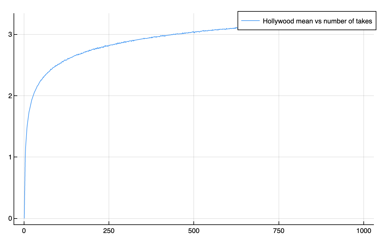
As we increase the number of takes, the mean of the Hollywood distribution grows at a logarithmic rate. We get diminishing returns from more and more takes.
And now for variance, how many different things the actor tries (I'll use the standard deviation instead):
n_deviations = 10
deviations = 1:n_deviations
gumbel_mean_by_deviation = zeros(n_deviations)
n_takes = 10
for d = deviations
    distribution = Normal(0, d)
    gumbel_mean_by_deviation[d] = mean(sample_gumbel(distribution, n_samples, n_takes))
end

plot(deviations, gumbel_mean_by_deviation, label="Hollywood mean vs std deviation")
We can see how the mean of the Hollywood distribution grows linearly as the "input" standard deviation grows:
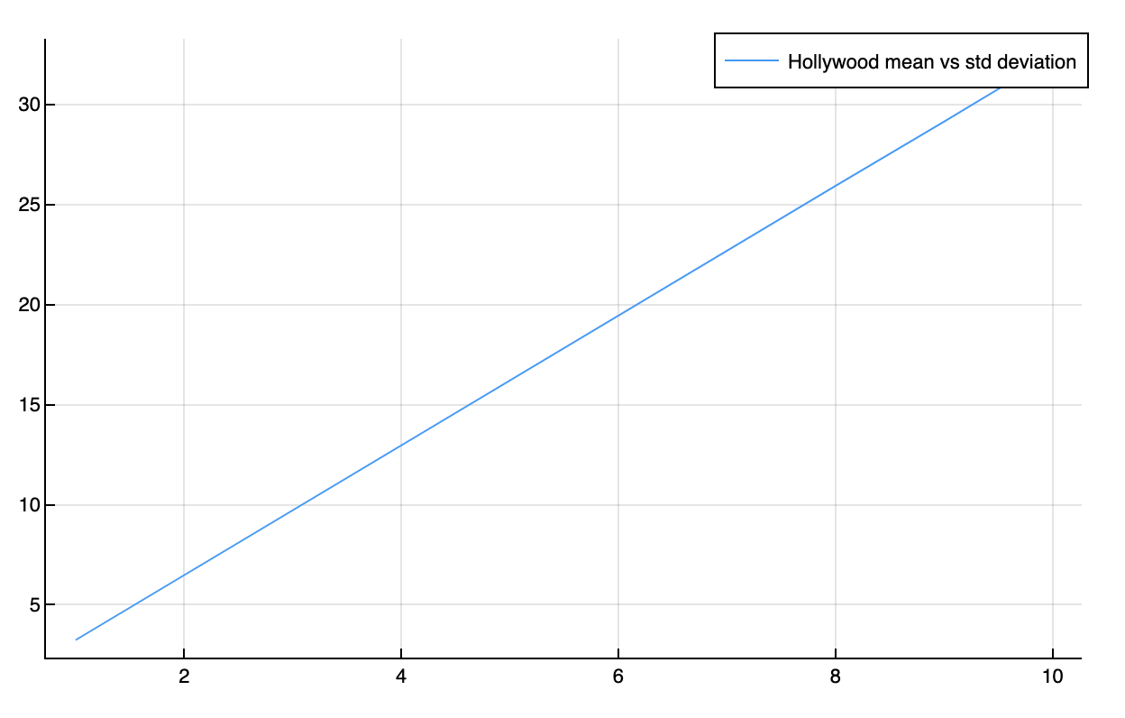
We get a lot of benefit from having crazy actors trying crazy things. The hope is that if the actors try crazier and crazier things, the movies get better and better, even if some of their takes are terrible!
The idea of increasing the number of takes indefinitely is not just theoretical. Directors will try lots of takes. For example, in a podcast episode, Ben Stiller and Adam Scott explain that they tried multiple ideas and 14 takes to land in the final one, which IMO is fantastic. And 14 is not that many. David Fincher asked Jake Gyllenhaal to do 50 takes for a particular scene.
Variance budget
The "increase the variance" argument doesn't only apply to one actor. It applies to every actor in the take.
But that introduces a problem: assuming that each actor's performance is decorrelated from the others, the more actors on screen, the more unlikely that they'll all have a great shot at the same time. If you have 12 actors in one shot, the probability that they'll have an above average shot is 1/2^12 ≈ 0.024%1. You'll need a lot of shots just to get something decent.
If the quality of a shot is determined by the worst actor in the shot (i.e. minimum), then you are guaranteed to do worse the more actors you add:
max_n_actors = 10
actors = 1:max_n_actors
gumbel_mean_by_actors = zeros(max_n_actors)
n_takes = 10
n_samples = 1000
for n_actors = actors
samples = zeros(n_samples)
for s = 1:n_samples
takes = zeros(n_takes)
for t = 1:n_takes
takes[t] = minimum(rand(hollywood, n_actors))
end
samples[s] = maximum(takes)
end
gumbel_mean_by_actors[n_actors] = mean(samples)
end
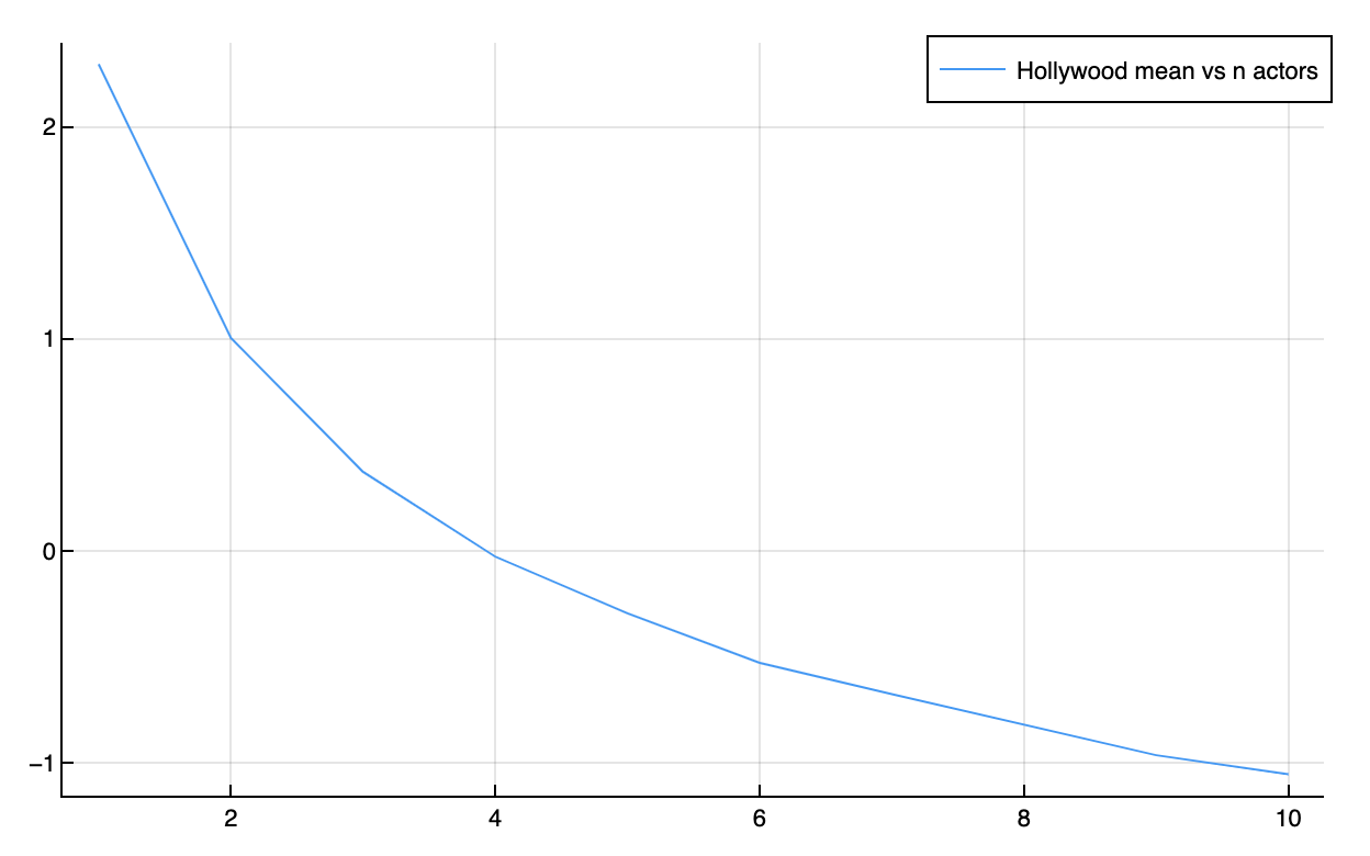
plot(actors, gumbel_mean_by_actors, label="Hollywood mean vs n actors")
You can see the mean shot getting worse and worse. In this case, variance is now your enemy:
Given that a software project can be ruined by a faulty part, it makes sense to have a variance budget that you should spend carefully, and only on factors that will multiply the final product.
Footnotes
- This and other "curses of dimensionality" are well-covered in chapter 9 of The Art of Science and Engineering.↩